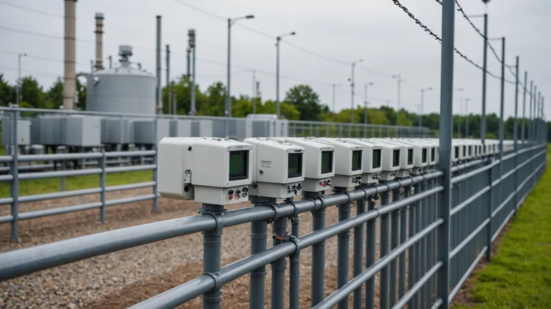
The hardest problem in continuous methane monitoring is not detection. With modern tunable diode laser absorption sensors or metal-oxide semiconductor sensors of sufficient sensitivity, measuring an elevated methane concentration is technically straightforward. The hard problem is answering the field question that follows detection: which specific component is leaking? An alert that says "elevated methane in the northwest sector" is useful for regulatory event logging, but it is not useful for a field crew who needs to know where to start looking. We think about source attribution as the part of the system that makes detection operationally useful rather than just regulatory documentation.
Why Radius-Only Detection Falls Short
Many commercial continuous monitoring systems produce alerts with a radius-based confidence zone: a circle of a defined size, centered on the emitting location, within which the source is estimated to be located. The radius size depends on the sensor network geometry and the atmospheric conditions at the time of detection. Under good conditions, the confidence radius might be 15 to 20 meters. Under variable wind conditions or at complex multicomponent sites, it can be 50 meters or more.
At a simple wellpad with a few primary components, a 20-meter radius might contain two or three fittings. That is manageable for a field inspection. At a compressor station with a typical equipment footprint, a 20-meter radius might contain 30 to 50 component connection points across multiple equipment strings. The field crew cannot inspect all of them in a single visit, and the prioritization of which components to inspect first is not well-informed by the radius alone. They are doing an improvised walk-down within the radius zone, which is faster than a full station walk-down but still much less efficient than going directly to the specific fitting.
The radius-only approach is also vulnerable to multi-source situations. If two components are emitting simultaneously within the same general area, a radius detection treats the combined signal as a single larger emission source. The attributed radius is centered somewhere between the two actual sources, potentially not pointing directly at either one. The field crew finding nothing at the center of the radius may conclude the alert was a false positive, when in fact there are two events that require separate investigation.
The Signal Processing Approach We Use
Our approach to source attribution combines two analytical layers that run on the multi-sensor concentration data. The first layer is cross-sensor correlation: comparing the timing, magnitude, and atmospheric persistence of concentration signals across multiple sensor nodes to establish which source area the plume is propagating from. In a sensor network where nodes are distributed around the perimeter and across the interior of a facility, the pattern of which sensors detected the event, at what relative timing, and at what relative magnitude contains directional information that a single sensor cannot provide.
The second layer applies an atmospheric dispersion model parameterized with the site-specific meteorological conditions at the time of the event. The concentration readings at each sensor location are the observable outputs of a dispersion process that started at the emission source. Working backward from the observed sensor readings to the most likely source location is an inverse dispersion calculation, sometimes called backward Lagrangian stochastic modeling in the research literature. The model iterates across possible source locations within the sensor network footprint and identifies the location that would produce the observed concentration pattern most closely, given the recorded wind speed, wind direction, atmospheric stability, and terrain.
The output is a probability map: a gridded representation of the facility with each grid cell assigned a probability of being the emission source, conditioned on the observed sensor data and atmospheric conditions. The cell with the highest probability is the primary attribution point. We report the attribution as a specific location with an uncertainty radius and a confidence qualifier, not as a single-point coordinate presented without uncertainty context. The field crew's dispatch information includes the primary location and the uncertainty bounds so they understand how precisely to anchor their initial inspection.
What Limits Attribution Accuracy
We want to be direct about the conditions under which our attribution accuracy is lower than the typical case, because operators making deployment decisions deserve an honest picture rather than a best-case scenario.
Calm or low-wind conditions, common during early morning hours, reduce attribution accuracy significantly. When wind speed is below roughly 1 meter per second, the dispersion pattern loses directional coherence. Gas meanders rather than forming a definite plume, and the concentration signal at sensors upwind versus downwind of the source becomes less discriminating. Under these conditions, the attribution confidence intervals widen substantially, and we reduce the confidence qualifier on the alert accordingly.
Complex terrain and obstructed airflow within dense equipment arrays disrupt atmospheric transport in ways that standard Gaussian dispersion models do not fully capture. A compressor station where the wind at sensor height is largely blocked by equipment enclosures and wind walls behaves differently from an open wellpad at the same geographic location. We address this with site-specific wind tunnel characterization during initial deployment calibration, but the residual uncertainty from flow obstruction is real and shows up in our confidence intervals.
Multiple simultaneous emission sources are more challenging to attribute individually than single-source events. When the sensor signal contains contributions from two or more distinct sources, the inverse dispersion calculation must partition the signal between them. With sufficient sensor density, this is often possible with reasonable confidence. With minimum sensor density configurations, multiple simultaneous events can result in a single attribution point located between the actual sources, which produces a false negative inspection outcome at each actual source location.
How Attribution Integrates with Field Dispatch
The attribution output feeds into our alert format, which includes a facility map image with the attribution probability overlay, the top three candidate component locations in rank order with their confidence scores, and the atmospheric conditions at the time of detection. When this goes to the field crew's mobile device, they can see the specific area of the facility flagged, zoom to the probability heat map overlay on their equipment layout, and navigate directly to the highest-probability component location.
In our early-access deployments, the difference in field resolution time between radius-only alerts and attribution-enriched alerts has been the most consistently valued improvement operators report. The practical issue on a busy compressor station is not that the crew cannot eventually find the leak; it is that finding it without directional attribution requires a substantial portion of a field shift. Attribution that narrows the search to a specific equipment string, rather than a quadrant, recovers several hours of field time per event, which compounds significantly over a monitoring subscription period at sites with non-trivial event rates.
Attribution is an Estimate, Not a Measurement
We want to close by being explicit about something that matters for how attribution data should be used. Source attribution from sensor array data using inverse dispersion modeling is an estimate. The model makes assumptions about atmospheric transport physics that hold approximately in most field conditions and less well in edge cases. The estimate's accuracy depends on the quality of the meteorological inputs, the density and calibration state of the sensor network, and the simplifying assumptions in the dispersion model.
An attribution result that points to "Rod Unit 2A packing area" should be understood as the most likely starting point for inspection, not as a certified declaration that the leak is at Rod Unit 2A. Field crews should inspect the attributed location first and then work outward if the initial inspection does not find the source. Treating attribution output as a definitive identification rather than a high-probability starting point is a misuse of the technology that will occasionally send a crew to the wrong place and erode confidence in the system. Treating it as what it is, a well-reasoned starting point, preserves its operational value and creates realistic expectations for what the technology contributes.
The signal processing methods and dispersion modeling approaches described in this article represent Aquanta Vision's current technical approach, which is under continuing development. Attribution accuracy metrics cited are from our early-access pilot deployments and reflect outcomes under the specific site configurations, sensor densities, and atmospheric conditions present at those sites. Results at other sites will depend on site-specific factors. These estimates are not certified measurements and are not intended as a substitute for direct component inspection or certified monitoring methods for regulatory reporting purposes.